Brain–Computer Interface with the Red Pitaya STEMLab 125-10

Overview

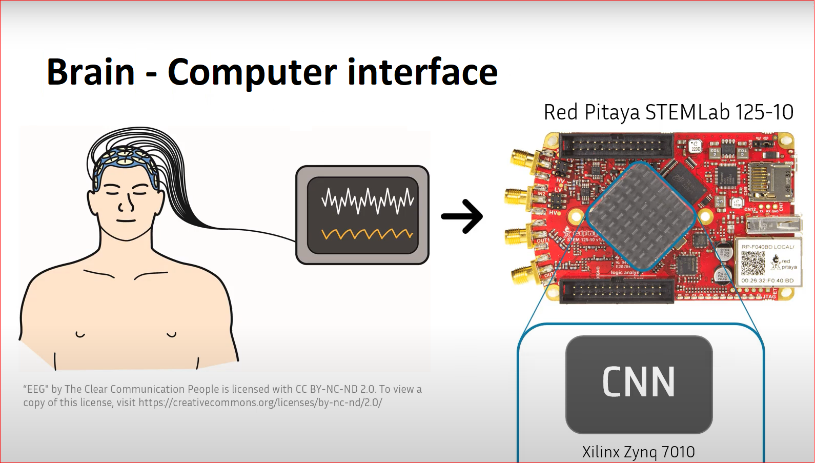
One of the most popular Brain-Computer Interface (BCI) paradigms is the motor imagery tasks’ recognition using electroencephalograph signals (EEG). One of the recently presented convolutional neural networks (CNNs) specifically designed to process EEG data is the EEGNet, that gets a good performance across different BCI paradigms while being compact enough to explore its implementation on edge devices. In this work, a EEGNet-based architecture has been implemented on the FPGA of the Xilinx Zynq 7010 system on-chip (SoC), the core of the Red Pitaya STEMlab 125-10. To achieve this, two optimization strategies have been explored: some data reduction techniques to control the size of the model and the fixed-point representation of the network.

Introduction

Brain-computer interfaces (BCIs) aim to enable direct communication between humans and computers by reading and identifying signals from the brain and acting on them. Their main inspiration comes from the medical field, but they have also applicability in entertainment and gaming systems, home automation or human enhancement.

Among all the BCI paradigms proposed throughout the field, we decided to focus on Motor Imagery (MI), a paradigm that consists on recognizing signals related to imagined movements. The commonly used brain-related signals for this paradigm are the electroencephalograph signals (EEG), which are easy to acquire and noninvasive. Traditionally, a combination of a feature extractor and a classifier has been used to process this type of signals and recognize the MI task, getting an acceptable level of performance. More recently, the convolutional neural networks (CNNs), which are a combination of these two types of algorithms, have been used to process EEG getting similar levels of performance while being simpler than other Machine Learning (ML) algorithms. An example of this is the EEGNet, a compact CNN architecture robust enough to learn a wide variety of interpretable features over a range of BCI tasks, with better generalization across paradigms than other reference algorithms.

Besides, when one thinks in the design of widely-used BCI, the processing algorithm is not the only point that must be taken into account, but also the hardware support that is going to run it. A possibility is to upload the EEG signals to the cloud and use the strong computational resources there to identify the MI task, but this would require an always-available Internet connection for the user, that would increase the battery consumption and could jeopardize their privacy, since their thoughts are being processed in a Big Tech datacenter. A solution to remove the Internet connection from the equation is to use the edge computing, meaning that all the computational load is processed on the user’s device. Of course, this will require of a stronger hardware in computational terms. There are a lot of hardware possibilities where the CNNs can be run, from the general-purpose and parallel-limited Central processing Units (CPUs) to the super-efficient Application-Specific Integrated Circuits (ASICs). The Field-Programmable Gate Arrays (FPGAs) are in a middle point, meeting a good balance between efficiency and flexibility. The Xilinx Zynq 7000 System on-Chip (SoC) series, as the 7010, present in the Red Pitaya STEMlab 125-10, specially stand out, since they have both a CPU and a FPGA, enabling the acceleration of functions on-chip while being easy to interface with, as they support light-weight Operative Systems as Red Pitaya OS.

In this project a EEGNet-based model has been adapted to work with the Physionet’s Motor Movement/Imagery dataset. Once trained, it has been implemented in the FPGA of the Xilinx Zynq 7010 SoC present in the STEMlab 125-10 board. To fit the model inside this compact FPGA, two strategies have been followed: (1) data reduction techniques have been applied to reduce the shape of the dataset elements, thus reducing the neural architecture’s size; and (2) fixed-point datatypes have been selected to represent the neural network values: inputs, parameters, feature maps and outputs.

Dataset

The Physionet Motor Movement/Imagery dataset was selected to train the models. This dataset includes 64-channels EEG recording of 105 valid subjects performing four different motor imagery tasks:

• Open and close the left fist (L)
• Open and close the right fist (R)
• Rest (0)
• Open and close both feet (F)

For comparison purposes, the commonly used criteria of 2-, 3- and 4-imagined-classes (L/R, R/L/0 and R/L/0/F, respectively) for this dataset was used. A total of 21 samples per class and subject are selected from the whole dataset, which are extracted in the stimuli window (Figure 1), where the subject must perform the corresponding motor imagery task for 4 seconds.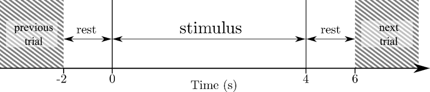

Figure 1: Trial timing scheme. Each stimulus is 4 s long and is 2 s apart from the previous and next one.

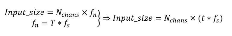
The input data shape is the number of channels, , times the number of frames, , which is computed by multiplying the time in seconds,, with the sampling frequency, , as described in the equations below:

The dependency between the input size and the model’s parameters determines the computational resources limitations for the FPGA implementation. To solve this issue, the data extraction strategies presented in this EEGNet MCU implementation work, were considered:

• Time window shortening: Since the stimulus firstly appears at (see Figure 1) the most relevant data should be concentrated close to the left side of the stimulus window. Removing data from the right side of the window should not result in accuracy loss, while significantly reducing the number of frames, and thus, the input size. This is the parameter, that will be either 1, 2 or 3 seconds.
• Data downsampling: As mentioned, the EEG recordings were sampled at 160 Hz, thus limiting the valuable information up to the 80 Hz due to Nyquist frequency. Physiology studies that have related the motor movement and imagery to the brain waves, show that these tasks are related to the µ and β waves, which range between 7.5 Hz and 30 Hz. Bearing this in mind, if a downsampling factor of two is applied (), the bandwidth is shortened to 40 Hz, with the µ and β waves still within it, while the number of frames is the half, . On the other hand, when the maximum frequency is 26.67 Hz, slightly cropping higher frequencies of the β wave and reducing three times the number of frames. In this manner, the input data and network’s parameters are reduced using downsampling.

Data augmentation is another possible advantage of using a downsampling technique. The commonly discarded frames are added to the data (Figure 2), multiplying the amount of patterns by a factor .

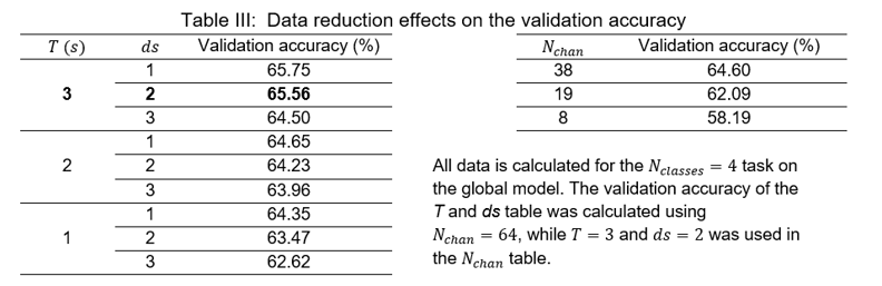
Channels reduction: As previously mentioned, the dataset provides 64-channels EEG signals. A channel reduction analysis aims to evaluate the model performance on different conditions. Moreover, it emulates other electrode’s configuration from other EEG acquisition systems. Three subsets of the initial 64 electrodes are set to be explored: 38, 19 and 8 (Figure 3). The 19 electrodes scenario corresponds to the 10-20 international system for EEG electrodes placement, while the 8 electrodes’ positions are the used in the Bitbrain’s minimal EEG caps. The 38 electrodes scenario represents a middle point between 64 and 19 electrodes configurations.

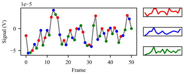Figure 2: Data augmentation technique used when the signal is downsampled. In this case ds=3, so each third subset of frames is treated as a sample.

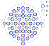
Figure 3: Electrodes’ map and its subdivisions. Image taken from here.

Model architecture

As mentioned in the introduction, the model architecture is based on the EEGNet, a CNN model that has demonstrated its versatility in various EEG-based paradigms while been compact enough to explore its implementation in hardware.

To meet our goals, the model’s architecture was fitted to the dataset according to the EEGNet original paper. However, three main changes were made to this architecture. First, the Exponential Linear Unit (ELU) was replaced by the Leaky Rectified Linear Unit (LeakyReLU), since this one is easier to be implemented in hardware while maintaining similar accuracy levels. Then, the alpha factor of the LeakyReLU was set to stepped values with the highest one at the first occurrence of the activation, 0.6, 0.5 and 0.4, respectively. Lastly, Dropout and Batch Normalization were removed. Moreover, the model must be adapted to the aforementioned data reduction methods. The resulting architecture combining the original EEGNet model, the proposed changes and the data extraction methods is the shown in Figure 4 and detailed in Table I.

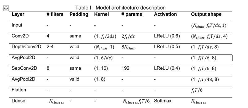
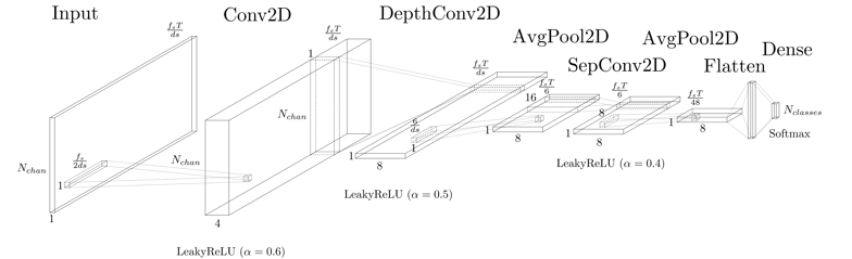
Figure 4: EEGNet-based model architecture visualization.

Model Training

Due to the inter- and intra-subject variance in the EEG signals for the same MI task, the training strategy followed in this work was splitted in two stages. First, a global model is trained over the entire dataset, and then transfer learning is applied to train subject-specific (SS) models using the global one as the starting-point.

The mentioned cross-validation technique used for evaluation was the same as the one presented in this work for the Physionet Motor Movement/Imagery dataset. This technique uses 5-fold to validate the global model, using one fifth of the subjects to validate each model fold and 4-fold for the subject-specific models, i.e., using one fourth of the trails of each subject to validate each SS model. A visualization of this cross-validation method is shown on Figure 5.

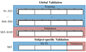Figure 5: Cross-validation method. In the global case, 5-fold cross-validation is done over the subjects, so each fold is validated using an iterating fifth of them, in this case the subjects 85-105. Once the global model is validated, the subject-specific models are trained using the global fold in which the subject that was used as validation. For the SS case, 4-fold cross validation is applied. Image taken from here.

The global model was implemented in Keras over Tensorflow 2.4.1 and trained for 100 epochs using a batch size of 16. Adam optimizer was selected, with a learning rate scheduler that decreases the learning rate by steps to 10^-2, 2·10^-3, 2·10^-4, 4·10^-6 and 4·10^-8 at epochs 0, 20, 40, 60 and 80, respectively. The SS-TL models were trained for 5 more epochs using the same fine-tuned hyperparameters except for the learning rate, which was fixed to 10^-2. An AMD Ryzen 5 3400G CPU at 3.7 GHz computer with a NVIDIA Quadro P2000 GPU with CUDA 11.2 was used for these simulations.

The results obtained for 2-, 3- and 4-classes classification tasks compared with other works using the Physionet Motor Movement/Imagery dataset can be found in Table II.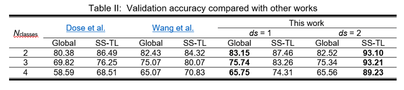

Apart from that, the results for different data-reduction scenarios are available in Table III.

The code for the data preparation, architecture definition and training process can be found in the training notebook of the project’s Github repo.

FPGA implementation

As commented above, the targeted FPGA is the XC7Z010, the PL of the Xilinx’s Zynq 7010 SoC present on the Red Pitaya STEMLab 125-10, which has 28 K programmable logic cells, 17.6 K look-up tables (LUTs), 35.2 K flip-flops (FF), 2.1 Mb of BRAM (block random-access memory) and 80 DSP (digital signal processing) slices of 18×25 MAC (multiplier-accumulator). This SoC includes a processing system based on a dual-core ARM Cortex-A9 with a maximum frequency of 667 MHz.

An algorithmic description of the implemented neural network was developed in C++, which can be found in the project’s Github repo. This code was used as the source for a Vivado High-level Synthesis project. To reduce the resource’s footprint, the design uses fixed-point datatypes to represent the network parameters, concretely <16,8>, meaning that 16 bits are used to represent numerical values, from which 8 correspond to the integer part representation. Due to the quantization effect present in the port of both the model parameters and the input data, from the Keras floating point representation into the selected fixed-point, an accuracy drop is expected when implementing the model in HLS.

To measure this accuracy loss, a HLS C simulation was run using the testbench that loads the model parameters and evaluates the validation set for each fold. The mean validation accuracy of the global model folds drops approximately 0.1 % (Figure 6).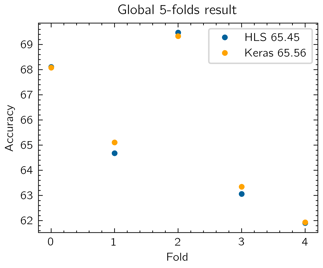

Figure 6: Validation accuracy for each fold when the model is virtualized in Keras (orange) and simulated its implementation in HLS (blue).

Once the HLS model was validated, it was synthetized. A pipeline directive was introduced in the inner loops of each layer, which significantly reduces the inference time (latency) of the FPGA implemented network from seconds to tens of milliseconds. Additionally, the interface directives were included to set all the ports as AXILite slave interfaces, enabling the communication with the Zynq Processing System through the AXI interface when loaded in the FPGA. The average time latency and the FPGA resources consumption for different data reduction scenarios are shown in Table IV.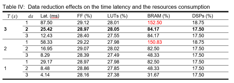

The and implementations (marked in red) were automatically discarded since they overconsume the available BRAM in the XC7Z010. Anyways, for the rest of the scenarios the model fits in the targeted FPGA. For this reason, the model was selected to be implemented in the FPGA since it gets the best accuracy while maintaining an acceptable inference time of 25 ms.

With the aim of automating the C simulation and synthesis operations, a small Python library which makes these processes callable from a higher-level language was developed, facilitating the exploration of all the data-reduction scenarios. Basically, it uses templates of the source files and the testbench that can be configured from Python to create them with the desired dataset parameters ( , and ). Additionally, since the validation of the dataset in the HLS simulated model takes too long, the developed Python code launches each fold separately as a background process, reducing the simulation time by a factor of 5. The use of these functions for simulating and synthetizing is included in the implementation notebook.

The Vivado IP integrator was used to implement the Vivado HLS-exported IP of the model, as shown in Figure 7. Using the block autoconnection feature of Vivado makes straight the integration of the IP containing the neural model into a block design with the Zynq Processing System.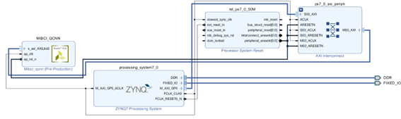

Figure 7: Block design that integrates the model IP (MIBCI_QCNN).

Once the IP is integrated, the bitstream is generated and loaded into the Red Pitaya together with the model parameters and the dataset through SFTP (Secured File Transfer Protocol). Red Pitaya automatically launches a Jupyter Notebooks server when booted, in which we are going to run the usage notebook. Table V contains the validation accuracy for the global model with , , and implemented in Keras, HLS and the FPGA.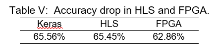

Conclusion and future work

An EEG-based FPGA implementation of a QCNN for MI tasks classification was presented in this project. The compact network was correctly trained and tested in Keras platform, as well as implemented using the Vivado HLS+Vivado IP integrator workflow on the Xilinx Zynq 7010. Additionally, a custom driver has been developed to control the model implemented on the FPGA from the SoC’s CPU. To fit the model in the FPGA, two methods have been used: the reduction of the dataset and the representation of the neural network with 16-bit fixed-point values.

The subject specific models achieve an average validation accuracy of 93.10 %, 93.21 % and 89.23 % for 2-, 3- and 4-class MI tasks classification. Moreover, the FPGA implementation has proven to have a minimum loss of 2.7 % of accuracy for our trained model, with expected response (latency) times of less than 30 ms.

Finally, the development of the complete FPGA-based BCI prototype is part of the second stage of this project. The neural model implemented into the FPGA will be used as the kernel of a low-cost real-time device that infers the patterns from the multiplexed EEG channels electronic signals connected to the coaxial input of the Red Pitaya development board.

For the full article click here.